프리미엄
예측대회
투자분석
아카데미
커뮤니티
로그인Valley AI 시작하기시작하기
Valley Space인기
퀀트 도전 - 월간 퀀트스터디, 옵션) SPX 옵션 분석하기(250304 코드 개선), LPPL 업데이트
Neurodoc퀀트

퀀트 도전 - 월간 퀀트스터디, 옵션) SPX 옵션 분석하기(250304 코드 개선), LPPL 업데이트

avatar
neurodoc
2025.03.02조회수 31회

WSAJ Premium - 독점 콘텐츠 | Valley AI
월간 퀀트 스터디 보고 오시면 좋습니다.

아래에 간략히 설명해뒀으니 그거만 보셔도 충분하긴해요


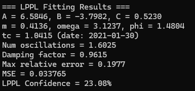
우선 LPPL로 crash도 분석해보면 좋을 것 같아서 업데이트했다.

업데이트한 코드는 문라이트에 남겨두겠다.

(이전 글로!)

image.png

오늘의 주제는 저번 달 퀀트 스터디인 S&P500 옵션 마켓메이커(MM)들의 포지션이 주식시장에 미치는 영향


옵션 시장에서 마켓 메이커(MM)가 어떻게 주식시장 변동성에 영향을 미치는지를 설명해주신 글이다

요약해보자면 아래와 같다

  1. 델타(Δ)

    • 기초자산(예: S&P500 지수)이 1만큼 움직일 때 옵션 가격이 얼마나 변하는지를 나타낸다.

    • 마켓 메이커(MM)는 고객과 거래할 때 생기는 옵션 포지션의 “델타 위험”을 없애려고, 기초자산을 사거나 팔면서 델타를 0으로 맞추려고 하고, 이를 ‘델타 헤징’이라고 부른다.

  2. 감마(Γ)

    • 델타가 얼마나 빨리 변하는지를 보는 지표입니다.

    • 감마가 크면 기초자산이 움직일 때마다 MM이 더 큰 규모로 헷지 매매를 해야 한다.

  3. 롱 감마 vs. 숏 감마

    • 롱 감마(+) 상태: 주가가 오르면 MM은 기초자산을 팔고, 주가가 내리면 사들이게 된다. 결과적으로 시장 변동성을 완화한다

    • 숏 감마(–) 상태: 주가가 오르면 더 사고, 내리면 더 파는 방향으로 매매가 이루어져 변동성이 커질 수 있다.
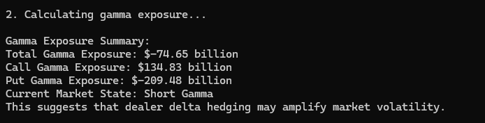
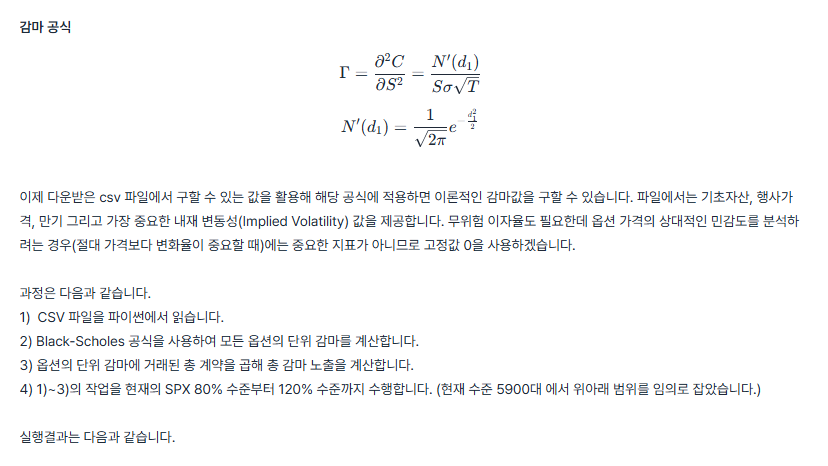
  4. 실제 데이터로 감마 노출도 계산

    • 감마 × 미결제약정 × 지수 × 계약단위 등을 합산해, MM 전체가 얼만큼 기초자산을 사고팔지 예상해볼 수 있다.

    • 만기별, 행사가격별로 감마가 얼마나 쌓여 있는지도 살피면, 시장이 특정 가격대에서 갑자기 출렁일지 예측하는 힌트를 얻을 수 있다.

  5. 감마 플립(Gamma Flip)

    • 어떤 지수 수준을 기점으로 시장 전체가 숏 감마에서 롱 감마로 바뀌는 구간을 뜻한다.

    • 예를 들어 지수가 5,900 근처일 때 숏 감마였다가, 5,985 이상으로 올라가면 롱 감마로 뒤집힌다면, 그 지점부터는 변동성이 줄어들 가능성이 커진다.

결국 이 글이 말해주는 건, “옵션 시장을 주시하면 주가의 단기 움직임(특히 변동성)에 대한 추가적인 단서를 얻을 수 있다”라는 점아다. 숏 감마면 시장이 더 크게 출렁이고, 롱 감마면 비교적 차분해진다는 것이 핵심 포인트
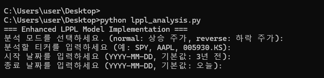

그래서 구현해봤다.


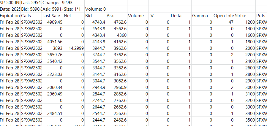
2025-03-02 기준 옵션 분포다.


image.png
image.png

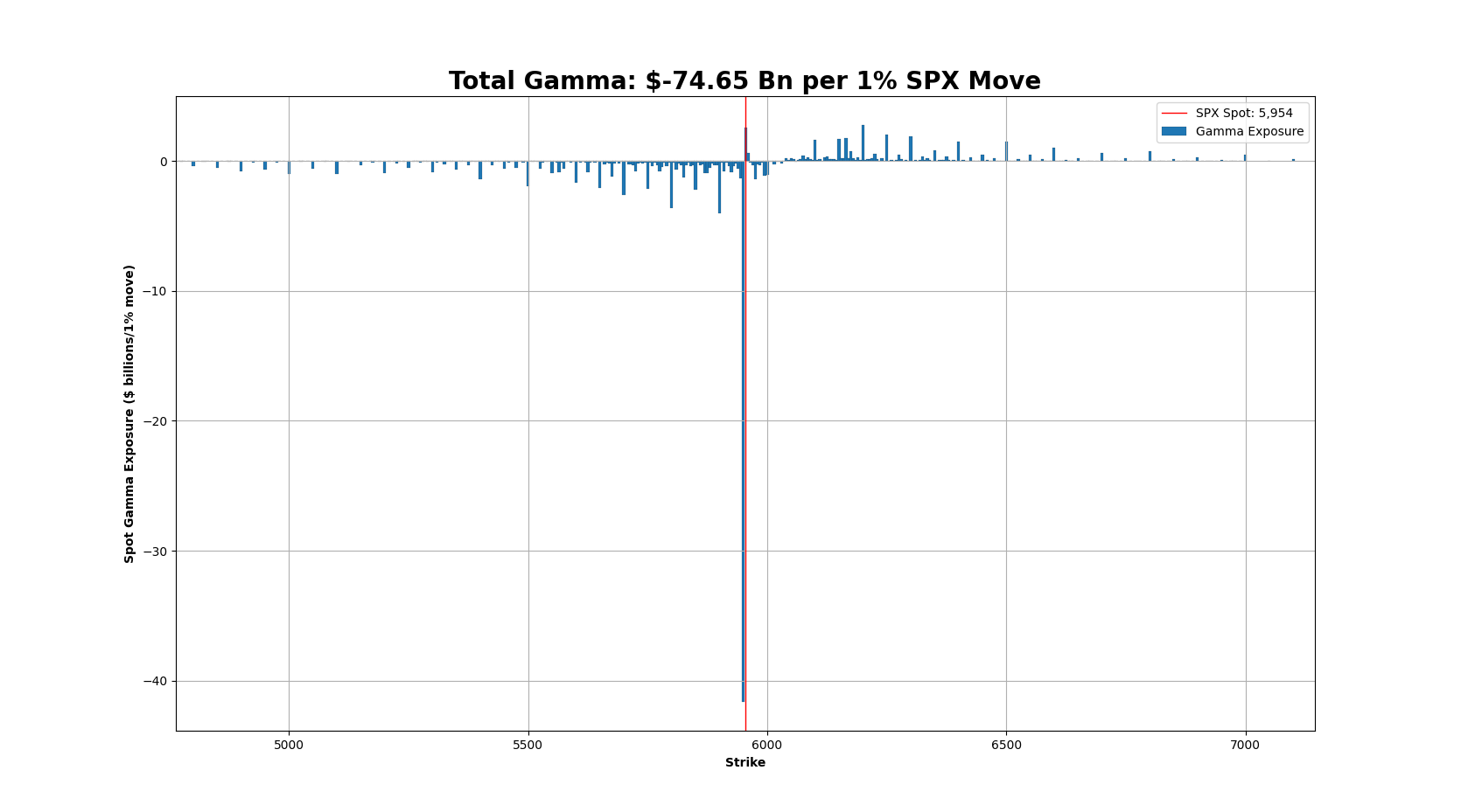
(Visualizing gamma by strike)

image.png

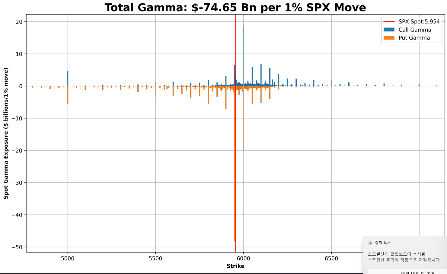
(Visualizing gamma by call/put)

현재는 숏 감마 상태로 변동성이 커질 수 있다.


image.png

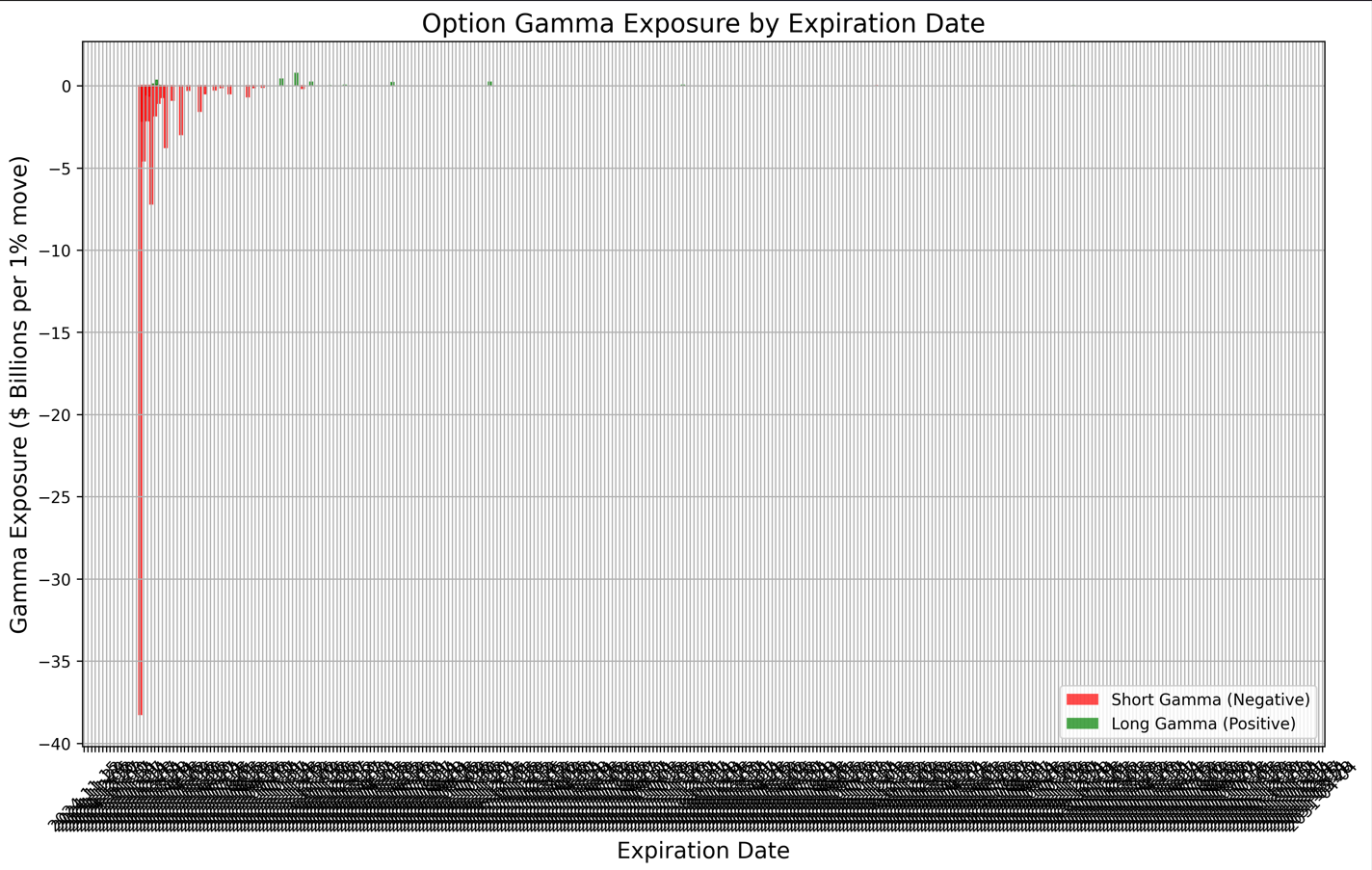
(Visualizing gamma by expiration)

가까운 만기일에 숏감마인 옵션이 많은 모습 (매 만기일 별로 표기했더니 난잡하다. 수정이 필요)


그런데 여기서부터 문제가 발생했다

image.png

?????? 내가 받은 파일에는 내재 변동성이 없던데?? 어떻게 구현하지?


답을 찾아 헤매던 중

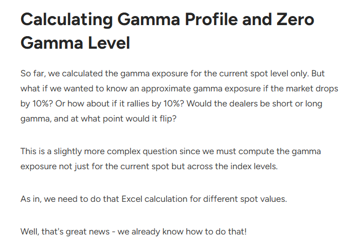
How to Calculate Gamma Exposure (GEX) and Zero Gamma Level

(감사합니다)

image.png
image.png

아... IV 이걸 못봤네..... 미치겠다

그래도 찾았으니 다행 다시 시작


그래서 현재 감마플립 포인트는 어디냐?

image.png

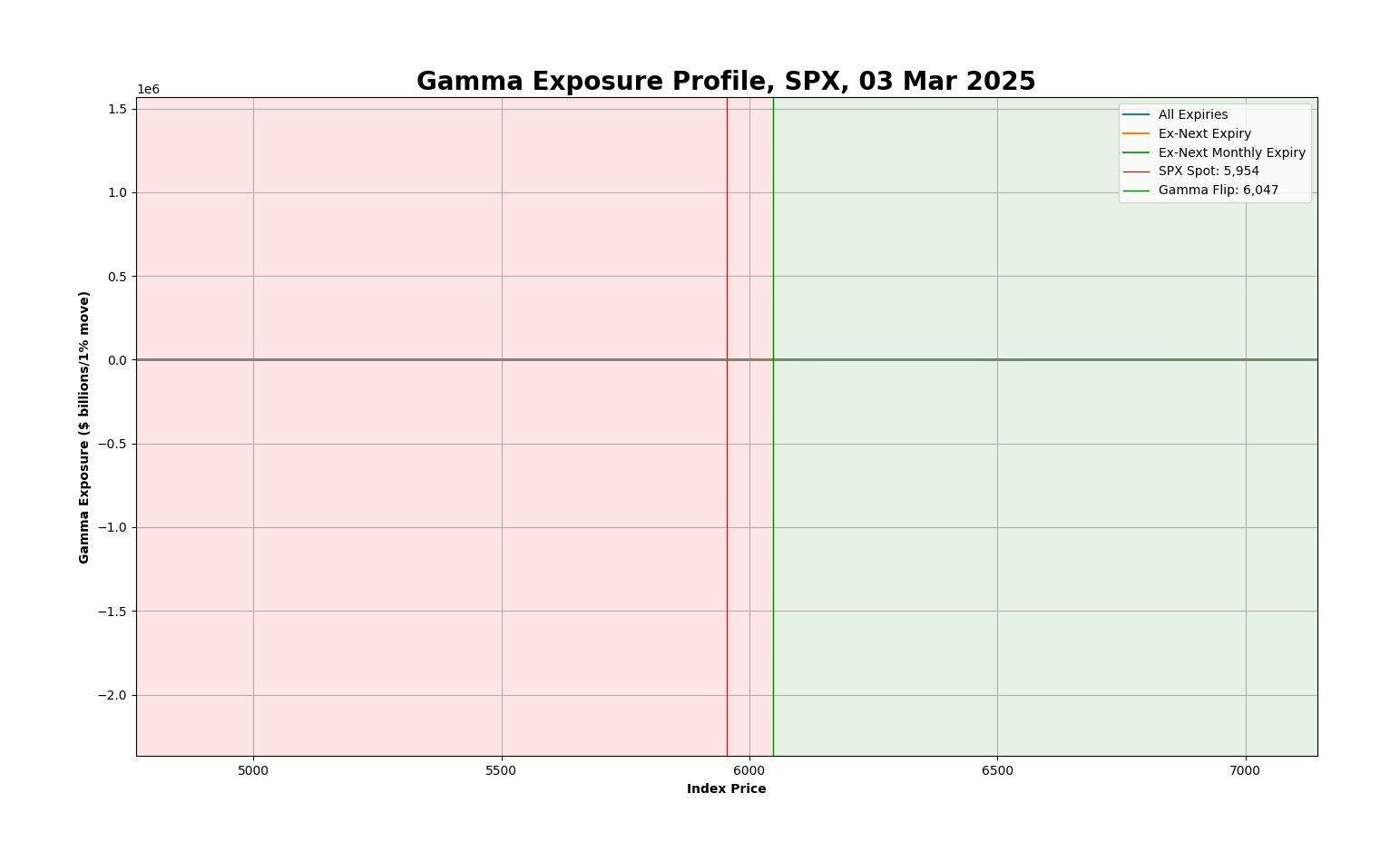
(Visualizing gamma profile)

현물: 5954.5

감마플립 포인트: 6049


저 위로 올라가야 시장 변동성이 좀 가라 앉겠구나 정도로 받아들이면 된다.

오늘의 코드 역시 문라이트에 공유드립니다. (스스로 검증해보고 쓰기)


그림 나오는게 마음에 안 들어서 수정할 예정


읽어주셔서 감사합니다.


(2025-03-04 업데이트 옵션 코드)

import pandas as pd
import numpy as np
import matplotlib.pyplot as plt
import matplotlib.dates as mdates
import os, re
from scipy.stats import norm
from datetime import datetime, timedelta, date
import requests

pd.options.display.float_format = '{:,.4f}'.format

# -----------------------------------#
# Black-Scholes 기반 감마 계산 함수   #
# -----------------------------------#
def black_scholes_delta_gamma(S, K, IV, T, r, sigma, option_type, open_interest):
    if T == 0 or IV == 0:
        return 0
    dp = (np.log(S/K) + (r - sigma + 0.5*IV**2)*T) / (IV*np.sqrt(T))
    dm = dp - IV*np.sqrt(T)
    if option_type == 'call':
        gamma = np.exp(-sigma*T) * norm.pdf(dp) / (S * IV * np.sqrt(T))
        return open_interest * 100 * S * S * 0.01 * gamma
    else:
        gamma = K * np.exp(-r*T) * norm.pdf(dm) / (S * S * IV * np.sqrt(T))
        return open_interest * 100 * S * S * 0.01 * gamma

# -----------------------------------#
# 안전한 데이터 변환 함수들            #
# -----------------------------------#
def safe_int_convert(s):
    try:
        if pd.isna(s):
            return 0
        return int(s)
    except (ValueError, TypeError):
        digits = ''.join(filter(str.isdigit, str(s)))
        return int(digits) if digits else 0

def safe_float_convert(s):
    try:
        if pd.isna(s):
            return 0.0
        return float(s)
    except (ValueError, TypeError):
        numeric_chars = re.sub(r'[^\d.]', '', str(s).replace(',', '.'))
        parts = numeric_chars.split('.')
        if len(parts) > 2:
            numeric_chars = parts[0] + '.' + ''.join(parts[1:])
        return float(numeric_chars) if numeric_chars else 0.0

# --------------------------------------------------#
# API에서 SPX 옵션 데이터 받아오기 및 전처리 함수      #
# --------------------------------------------------#
def fetch_spx_options_data(index):
    url = "https://cdn.cboe.com/api/global/delayed_quotes/options/_" + index + ".json"
    print(f"Fetching data from API: {url}")
    response = requests.get(url)
    options = response.json()
    
    # 스팟 가격 및 오늘 날짜 추출
    spot_price = options["data"]["close"]
    today_date = date.today()
    
    # 옵션 데이터를 DataFrame으로 변환
    data_df = pd.DataFrame(options["data"]["options"])
    
    # 옵션 문자열에서 콜/풋, 만기, 행사가격 추출
    data_df['CallPut'] = data_df['option'].str.slice(start=-9, stop=-8)
    data_df['ExpirationDate'] = data_df['option'].str.slice(start=-15, stop=-9)
    data_df['ExpirationDate'] = pd.to_datetime(data_df['ExpirationDate'], format='%y%m%d', errors='coerce')
    data_df['Strike'] = data_df['option'].str.slice(start=-8, stop=-3)
    data_df['Strike'] = data_df['Strike'].str.lstrip('0')
    
    # 콜과 풋 데이터 분리 후 재정렬
    data_df_calls = data_df.loc[data_df['CallPut'] == "C"].reset_index(drop=True)
    data_df_puts = data_df.loc[data_df['CallPut'] == "P"].reset_index(drop=True)
    
    df = data_df_calls[['ExpirationDate','option','last_trade_price','change','bid','ask','volume','iv','delta','gamma','open_interest','Strike']]
    df_puts = data_df_puts[['ExpirationDate','option','last_trade_price','change','bid','ask','volume','iv','delta','gamma','open_interest','Strike']]
    df_puts.columns = ['put_exp','put_option','put_last_trade_price','put_change','put_bid','put_ask','put_volume','put_iv','put_delta','put_gamma','put_open_interest','put_strike']
    
    df = pd.concat([df, df_puts], axis=1)
    df['check'] = np.where((df['ExpirationDate'] == df['put_exp']) & (df['Strike'] == df['put_strike']), 0, 1)
    if df['check'].sum() != 0:
        print("PUT CALL MERGE FAILED - OPTIONS ARE MISMATCHED.")
        exit()
    df.drop(['put_exp', 'put_strike', 'check'], axis=1, inplace=True)
    
    df.columns = ['ExpirationDate','Calls','CallLastSale','CallNet','CallBid','CallAsk','CallVol',
                  'CallIV','CallDelta','CallGamma','CallOpenInt','StrikePrice','Puts','PutLastSale',
                  'PutNet','PutBid','PutAsk','PutVol','PutIV','PutDelta','PutGamma','PutOpenInt']
    
    # 데이터 타입 변환 및 시간 보정 (만기일 오후 4시로 고정)
    df['StrikePrice'] = df['StrikePrice'].astype(float)
    df['ExpirationDate'] = df['ExpirationDate'] + timedelta(hours=16)
    df['CallIV'] = pd.to_numeric(df['CallIV'], errors='coerce').fillna(0.001).clip(lower=0.001)
    df['PutIV'] = pd.to_numeric(df['PutIV'], errors='coerce').fillna(0.001).clip(lower=0.001)
    df['CallGamma'] = pd.to_numeric(df['CallGamma'], errors='coerce').fillna(0)
    df['PutGamma'] = pd.to_numeric(df['PutGamma'], errors='coerce').fillna(0)
    ...

회원가입만 해도
이 글을 무료로 읽을 수 있어요.

Basic 7일 무료 체험 시작하기
이미 계정이 있으신가요?로그인하기
댓글 2개
avatar
neurodoc
구독자 69명구독중 35명
훌륭한 의사이면서 좋은 투자자가 되길 꿈꿉니다
avatar
붐붐
2025.04.01

감사합니다! 단순복사해서 긁었는데, 이렇게 에러가 나오는데,, 어떤 부분이 잘못됐는지 모르겠습니다 (방화벽?) Failed to load data. Please try refreshing or check your internet connection.

퀀트 카테고리의 다른글

LPPL 코드 가져가셨던 분들 꼭 봐주세요!! (2025-03-03 추가 업데이트)

경량화 해서 트레이딩뷰에서 돌리려고 숫자 줄여봤던 부분이 남아있어서 full LPPL로 코드 수정해서 올립니다. 이전에 가져가신 분들인 500이랑 20으로 서치하셔서 500 -> 750, 20->5로 바꾸시면 됩니다. 이전 글에 수정해서 코드 올려뒀으니 이전 글 다시 확인하셔도 됩니다 2025-03-03 LPPL 하락 분석 업데이트 import numpy as np import pandas as pd import yfinance as yf import matplotlib.pyplot as plt plt.rcParams['font.family'] ='Malgun Gothic' plt.rcParams['axes.unicode_minus'] =False from scipy.optimize import minimize from scipy.linalg import lstsq from datetime import datetime, timedelta import warnings import os import time import random warnings.filterwarnings('ignore') class LPPL: def __init__(self, observations): """ LPPL 모델 초기화 observations: DatetimeIndex와 'Adj Close' 열을 포함한 DataFrame. """ self.observations = observations.sort_index() self.t = self.get_days_since_start() self.price = self.observations['Adj Close'].values self.log_price = np.log(self.price) self.ts = self.t / self.t[-1] # [0, 1] 범위로 스케일링 # 파라미터 bounds 설정 self.bounds = { 'm': (0.1, 0.9), 'omega': (2, 25), 'phi': (0, 2 * np.pi) } # 유전 알고리즘 설정 self.population_size = 200 self.generations = 100 self.crossover_rate = 0.7 self.mutation_rate = 0.1 self.elitism_rate = 0.1 def get_days_since_start(self): """ DatetimeIndex를 시작 날짜로부터 경과한 일수 배열로 변환. """ start_date = self.observations.index[0] return (self.observations.index - start_date).days.values def lppl_matrix(self, t, tc, m, omega, phi): """ 주어진 파라미터로 LPPL 행렬 생성. """ t = np.array(t) dt = (tc - t).clip(0.00001) # 0에 가까워지는 수치적 문제 방지 dt_pow_m = dt ** m oscillatory = dt_pow_m * np.cos(omega * np.log(dt) - phi) return np.vstack((np.ones_like(t), dt_pow_m, oscillatory)).T def _func_(self, params, t, log_price): """ 비선형 최적화를 위한 목적 함수. """ m, omega, phi, tc = params try: lppl_m = self.lppl_matrix(t, tc, m, omega, phi) coefs = lstsq(lppl_m, log_price)[0] return np.sum((log_price - lppl_m @ coefs) ** 2) except (np.linalg.LinAlgError, ValueError): return 1e10 def simple_model_fit(self): """ 단순 모델 피팅(C=0, beta=1)으로 초기 tc 추정. """ t_end = self.ts[-1] def simple_obj(tc_val, t, log_price): dt = tc_val - t X = np.vstack((np.ones_like(t), dt)).T try: coefs = lstsq(X, log_price)[0] return np.sum((log_price - X @ coefs) ** 2) except np.linalg.LinAlgError: return 1e10 tc_candidates = np.linspace(t_end + 0.01, t_end + 0.1, 100) errors = [simple_obj(tc_val, self.ts, self.log_price) for tc_val in tc_candidates] best_tc = tc_candidates[np.argmin(errors)] dt = best_tc - self.ts X = np.vstack((np.ones_like(self.ts), dt)).T try: A, B = lstsq(X, self.log_price)[0] except np.linalg.LinAlgError: A = np.mean(self.log_price) B = -0.01 return best_tc, float(A), float(B) def initialize_population(self, tc_seed): """ 유전 알고리즘 초기 개체군 생성. """ population = [] t_end = self.ts[-1] tc_low, tc_high = t_end + 0.01, t_end + 0.1 initial_individual = np.array([ np.random.uniform(*self.bounds['m']), np.random.uniform(*self.bounds['omega']), np.random.uniform(*self.bounds['phi']), tc_seed ]) fitness = self._func_(initial_individual, self.ts, self.log_price) population.append((initial_individual, fitness)) for _ in range(self.population_size - 1): individual = np.array([ np.random.uniform(*self.bounds['m']), np.random.uniform(*self.bounds['omega']), np.random.uniform(*self.bounds['phi']), np.random.uniform(tc_low, tc_high) ]) fitness = self._func_(individual, self.ts, self.log_price) population.append((individual, fitness)) return population def tournament_selection(self, population, tournament_size=3): tournament = random.sample(population, min(tournament_size, len(population))) return min(tournament, key=lambda x: x[1]) def crossover(self, parent1, parent2): alpha = np.random.random() return alpha * parent1 + (1 - alpha) * parent2 def mutate(self, individual): m_strength = (self.bounds['m'][1] - self.bounds['m'][0]) * 0.1 omega_strength = (self.bounds['omega'][1] - self.bounds['omega'][0]) * 0.1 phi_strength = (self.bounds['phi'][1] - self.bounds['phi'][0]) * 0.1 tc_strength = 0.005 result = individual.copy() if np.random.random() < 0.3: result[0] = np.clip(result[0] + np.random.normal(0, m_strength), *self.bounds['m']) if np.random.random() < 0.3: result[1] = np.clip(result[1] + np.random.normal(0, omega_strength), *self.bounds['omega']) if np.random.random() < 0.3: result[2] = np.clip(result[2] + np.random.normal(0, phi_strength), *self.bounds['phi']) if np.random.random() < 0.3: t_end = self.ts[-1] tc_low, tc_high = t_end + 0.01, t_end + 0.1 result[3] = np.clip(result[3] + np.random.normal(0, tc_strength), tc_low, tc_high) return result def genetic_algorithm_fit(self, tc_seed): """ 유전 알고리즘을 이용한 LPPL 파라미터 최적화. """ population = self.initialize_population(tc_seed) best_params, best_fitness = min(population, key=lambda x: x[1]) for generation in range(self.generations): population.sort(key=lambda x: x[1]) elite_count = max(1, int(self.population_size * self.elitism_rate)) new_population = population[:elite_count].copy() while len(new_population) < self.population_size: if np.random.random() < self.crossover_rate: parent1 = self.tournament_selection(population)[0] parent2 = self.tournament_selection(population)[0] child = self.crossover(parent1, parent2) if np.random.random() < self.mutation_rate: child = self.mutate(child) fitness = self._func_(child, self.ts, self.log_price) new_population.append((child, fitness)) else: new_population.append(self.tournament_selection(population)) population = new_population[:self.population_size] current_best, current_fitness = min(population, key=lambda x: x[1]) if current_fitness < best_fitness: best_params, best_fitness = current_best, current_fitness # 개선이 없으면 조기 종료 if generation > 10 and abs(current_fitness - best_fitness) < 1e-6: break return best_params, best_fitness def multi_run_genetic_algorithm(self, tc_seed, runs=3): best_overall_params = None best_overall_fitness = float('inf') original_mutation_rate = self.mutation_rate original_population_size = self.population_size for run in range(runs): print(f"유전 알고리즘 실행 {run+1}/{runs}...") self.mutation_rate = original_mutation_rate + (run * 0.05) self.population_size = original_population_size + (run * 50) params, fitness = self.genetic_algorithm_fit(tc_seed) if fitness < best_overall_fitness: best_overall_fitness = fitness best_overall_params = params self.mutation_rate = original_mutation_rate self.population_size = original_population_size return best_overall_params, best_overall_fitness def fine_tune_parameters(self, params): """ 지역 최적화를 통한 파라미터 미세 조정. """ tuned_params = params.copy() param_bounds = [ self.bounds['m'], self.bounds['omega'], self.bounds['phi'], (self.ts[-1] + 0.01, self.ts[-1] + 0.1) ] for idx in range(4): def objective(x): params_copy = tuned_params.copy() params_copy[idx] = x[0] return self._func_(params_copy, self.ts, self.log_price) result = minimize(objective, x0=[tuned_params[idx]], bounds=[param_bounds[idx]], method='L-BFGS-B') if result.success: tuned_params[idx] = result.x[0] return tuned_params def verify_oscillations(self, params): """ 로그 주기적 진동의 유의미성을 확인. """ try: num_oscillations = float(params['num_oscillations']) damping_factor = float(params['damping_factor']) if num_oscillations >= 2.0: return True if damping_factor >= 0.8: return True tc, m, omega, phi = params['tc'], params['m'], params['omega'], ...
퀀트
2025. 03. 01
4
0
20

퀀트 도전- 월간 퀀트스터디, LPPL) 파이썬 LPPL 코드로 과거 TSLA 주가 분석해보기(코드 수정됐으니 받아가신 분들 필독!!)

*****경량화 해서 트레이딩뷰에서 돌리려고 숫자 줄여봤던 부분이 남아있어서 full LPPL로 코드 수정해서 올립니다. 글 내용도 수정됨***** 2019-01-01 ~ 2021-01-01 까지 TSLA 수정 종가를 바탕으로 한 분석 결과입니다. LPPL Confidence 23.08로 시장 과열에 가까운 경고단계 Critical time은 2021-01-30로 나왔습니다 이후 진짜로 그 쯤에서 버블이 꺼졌네요 자산군에 적용하는 것이 좋지만 만든김에 검증용으로 과거 테슬라 차트에 분석해봤습니다. 추가로 이미 퀀트팀에서 해주셨지만 SPY에 적용해볼까요? 오늘 날짜로 SPY는 LPPL confidence 6.38%로 주의필요 초기단계 쯤 되네요 앞으로 종종 모델 구현해서 공유해드리겠습니다. 아래는 만들어 본 코드입니다.(수정됨) valley fellow 분들만 재미로 사용해보셨으면 합니다! import numpy as np import pandas as pd import yfinance as yf import matplotlib.pyplot as plt from scipy.optimize import minimize from scipy.linalg import lstsq from datetime import datetime, timedelta import warnings import os import time import random warnings.filterwarnings('ignore') class LPPL: def __init__(self, observations): """ Initialize the LPPL model with historical price observations. Args: observations (pd.DataFrame): DataFrame with a DatetimeIndex and 'Adj Close' column. """ self.observations = observations.sort_index() self.t = self.get_days_since_start() self.price = self.observations['Adj Close'].values self.log_price = np.log(self.price) # Scale time array to [0, 1] for optimization purposes self.ts = self.t / self.t[-1] # Parameter bounds based on typical LPPL references self.bounds = { 'm': (0.1, 0.9), 'omega': (2, 25), 'phi': (0, 2 * np.pi) # tc bounds will be set dynamically during fitting } # Genetic algorithm settings self.population_size = 200 self.generations = 100 self.crossover_rate = 0.7 self.mutation_rate = 0.1 self.elitism_rate = 0.1 def get_days_since_start(self): """ Convert the DatetimeIndex into an array of days since the start date. Returns: np.ndarray: Array of days elapsed since the first date. """ start_date = self.observations.index[0] return (self.observations.index - start_date).days.values def lppl_matrix(self, t, tc, m, omega, phi): """ Construct the LPPL matrix for the given parameters. Args: t (np.ndarray): Scaled time array [0, 1]. tc (float): Critical time. m (float): Bubble growth exponent (equivalent to beta in literature). omega (float): Angular frequency of oscillations. phi (float): Phase shift. Returns: np.ndarray: LPPL matrix of shape (n, 3). """ t = np.array(t) dt = (tc - t).clip(0.00001) # Avoid numerical instability near zero dt_pow_m = dt ** m oscillatory = dt_pow_m * np.cos(omega * np.log(dt) - phi) return np.vstack((np.ones_like(t), dt_pow_m, oscillatory)).T def _func_(self, params, t, log_price): """ Objective function for non-linear parameter optimization. Args: params (np.ndarray): Parameter array [m, omega, phi, tc]. t (np.ndarray): Scaled time array. log_price (np.ndarray): Log of the price series. Returns: float: Sum of squared errors. """ m, omega, phi, tc = params try: lppl_m = self.lppl_matrix(t, tc, m, omega, phi) coefs = lstsq(lppl_m, log_price)[0] return np.sum((log_price - lppl_m @ coefs) ** 2) except (np.linalg.LinAlgError, ValueError): return 1e10 # Large penalty on error def simple_model_fit(self): """ Phase 1: Fit a simple model (C=0, beta=1) to obtain an initial seed for tc. Returns: tuple: (tc, A, B) as initial guesses. """ t_end = self.ts[-1] def simple_obj(tc_val, t, log_price): dt = tc_val - t X = np.vstack((np.ones_like(t), dt)).T try: coefs = lstsq(X, log_price)[0] return np.sum((log_price - X @ coefs) ** 2) except np.linalg.LinAlgError: return 1e10 # Set tc candidates from t_end + 0.01 to t_end + 0.1 (per strict criteria) tc_candidates = np.linspace(t_end + 0.01, t_end + 0.1, 100) errors = [simple_obj(tc_val, self.ts, self.log_price) for tc_val in tc_candidates] best_tc = tc_candidates[np.argmin(errors)] # Solve for A, B with best_tc dt = best_tc - self.ts X = np.vstack((np.ones_like(self.ts), dt)).T try: A, B = lstsq(X, self.log_price)[0] except np.linalg.LinAlgError: A = np.mean(self.log_price) B = -0.01 return best_tc, float(A), float(B) def initialize_population(self, tc_seed): """ Phase 2: Initialize the population for the genetic algorithm. Modified: Set tc range to [t_end + 0.01, t_end + 0.1]. Args: tc_seed (float): Initial tc seed from Phase 1. Returns: list: A list of tuples (params, fitness). """ population = [] t_end = self.ts[-1] tc_low, tc_high = t_end + 0.01, t_end + 0.1 # First individual using tc_seed initial_individual = np.array([ np.random.uniform(*self.bounds['m']), np.random.uniform(*self.bounds['omega']), np.random.uniform(*self.bounds['phi']), tc_seed ]) fitness = self._func_(initial_individual, self.ts, self.log_price) population.append((initial_individual, fitness)) # Remaining individuals for _ in range(self.population_size - 1): individual = np.array([ np.random.uniform(*self.bounds['m']), np.random.uniform(*self.bounds['omega']), np.random.uniform(*self.bounds['phi']), np.random.uniform(tc_low, tc_high) ]) fitness = self._func_(individual, self.ts, self.log_price) population.append((individual, fitness)) return population def tournament_selection(self, population, tournament_size=3): """Tournament selection for the genetic algorithm.""" tournament = random.sample(population, min(tournament_size, len(population))) return min(tournament, key=lambda x: x[1]) def crossover(self, parent1, parent2): """Crossover operation.""" alpha = np.random.random() return alpha * parent1 + (1 - alpha) * parent2 def mutate(self, individual): """Mutation operation.""" m_strength = (self.bounds['m'][1] - self.bounds['m'][0]) * 0.1 omega_strength = (self.bounds['omega'][1] - self.bounds['omega'][0]) * 0.1 phi_strength = (self.bounds['phi'][1] - self.bounds['phi'][0]) * 0.1 tc_strength = 0.005 # Mutation strength for tc result = individual.copy() if np.random.random() < 0.3: result[0] = np.clip(result[0] + np.random.normal(0, m_strength), *self.bounds['m']) if np.random.random() < 0.3: result[1] = np.clip(result[1] + np.random.normal(0, omega_strength), *self.bounds['omega']) if np.random.random() < 0.3: result[2] = np.clip(result[2] + np.random.normal(0, phi_strength), *self.bounds['phi']) if np.random.random() < 0.3: t_end = self.ts[-1] tc_low, tc_high = t_end + 0.01, t_end + 0.1 result[3] = np.clip(result[3] + np.random.normal(0, tc_strength), tc_low, tc_high) return result def genetic_algorithm_fit(self, tc_seed): """ Phase 2-3: Optimize LPPL parameters using the genetic algorithm. Args: tc_seed (float): Initial tc seed from Phase 1. Returns: tuple: (best_params, best_fitness) """ population = self.initialize_population(tc_seed) best_params, best_fitness = min(population, key=lambda x: x[1]) for generation in range(self.generations): population.sort(key=lambda x: x[1]) elite_count = max(1, int(self.population_size * self.elitism_rate)) new_population = population[:elite_count].copy() while len(new_population) < self.population_size: if np.random.random() < self.crossover_rate: parent1 = self.tournament_selection(population)[0] parent2 = self.tournament_selection(population)[0] child = self.crossover(parent1, parent2) if np.random.random() < self.mutation_rate: child = self.mutate(child) fitness = self._func_(child, self.ts, self.log_price) new_population.append((child, fitness)) else: new_population.append(self.tournament_selection(population)) population = new_population[:self.population_size] current_best, current_fitness = min(population, key=lambda x: x[1]) if current_fitness < best_fitness: best_params, best_fitness = current_best, current_fitness # Early stopping if no improvement after 10 generations if generation > 10 and abs(current_fitness - best_fitness) < 1e-6: break return best_params, best_fitness def multi_run_genetic_algorithm(self, tc_seed, runs=3): """ Run the genetic algorithm multiple times to find the best result. Args: tc_seed (float): Initial tc seed from Phase 1. runs (int): Number of runs. Returns: tuple: (best_params, best_fitness) """ best_overall_params = None best_overall_fitness = float('inf') original_mutation_rate = self.mutation_rate original_population_size = self.population_size for run in range(runs): print(f"Genetic Algorithm run {run+1}/{runs}...") self.mutation_rate = original_mutation_rate + (run * 0.05) self.population_size = original_population_size + (run * 50) params, fitness = self.genetic_algorithm_fit(tc_seed) if fitness < best_overall_fitness: best_overall_fitness = fitness best_overall_params = params self.mutation_rate = original_mutation_rate self.population_size = original_population_size return best_overall_params, best_overall_fitness def fine_tune_parameters(self, params): """ Phase 3: Fine-tune parameters using local optimization. Modified: Set tc bounds to [t_last + 0.01, t_last + 0.1]. Args: params (np.ndarray): Initial parameters [m, omega, phi, tc]. Returns: np.ndarray: Refined parameters. """ tuned_params = params.copy() param_bounds = [ self.bounds['m'], self.bounds['omega'], self.bounds['phi'], (self.ts[-1] + 0.01, self.ts[-1] + 0.1) ] for idx in range(4): def objective(x): params_copy = tuned_params.copy() params_copy[idx] = x[0] return self._func_(params_copy, self.ts, self.log_price) result = minimize(objective, ...

실패한? LPPL 파이썬 코드입니다

모든 시점에 모든 자산에서 0%가 나오는 듯... ㅠㅜ 어쩌면 야후 파이낸스 데이터 문제일지도 일단 도전해봤다는 것에 의의를 둡니다 import numpy as np import pandas as pd import yfinance as yf import matplotlib.pyplot as plt from scipy.optimize import minimize from scipy.linalg import lstsq from datetime import datetime, timedelta import warnings import os import time warnings.filterwarnings('ignore') class LPPL: def __init__(self, observations): """ LPPL 모델 초기화. Parameters: observations (pd.DataFrame): 'Close' 가격 데이터와 DatetimeIndex를 포함하는 DataFrame. """ self.observations = observations self.t = self.get_days_since_start() # 시작일로부터의 일수 계산 self.price = self.observations['Close'].values self.log_price = np.log(self.price) self.ts = self.t / self.t[-1] # 최적화를 위해 t를 [0,1] 범위로 스케일 조정 self.bounds = [ (0.01, 0.99), # m의 범위 (6, 13), # omega의 범위 (0, 2 * np.pi), # phi의 범위 # tc의 범위는 fit()에서 추가 ] def get_days_since_start(self): """ DatetimeIndex를 시작일로부터의 일수 배열로 변환. Returns: np.array: 시작일로부터의 일수를 나타내는 정수 배열. """ start_date = self.observations.index[0] return (self.observations.index - start_date).days.values def lppl_matrix(self, t, tc, m, omega, phi): """ 주어진 파라미터에 대해 LPPL 행렬을 계산. 이 버전은 다음과 같은 3항식 형태를 사용합니다: log(p(t)) = A + B*(tc-t)^m + C*(tc-t)^m * cos(omega * log(tc-t) - phi) Args: t (np.ndarray): 스케일 조정된 시간 배열 (0~1). tc (float): 임계 시간. m (float): 버블 성장 지수. omega (float): 진동 주파수. phi (float): 위상 이동. Returns: np.ndarray: (n, 3) 모양의 LPPL 행렬. """ t = np.array(t) dt = (tc - t).clip(0) # 음수가 되지 않도록 함 dt_pow_m = dt**m oscillatory = dt_pow_m * np.cos(omega * np.log(dt + 1e-8) - phi) return np.vstack((np.ones_like(t), dt_pow_m, oscillatory)).T def _func_(self, x, *args): """ 최적화에서 최소화할 목적 함수 (비선형 파라미터에 대해). Args: x (np.ndarray): 비선형 파라미터 [m, omega, phi, tc] 배열. *args: 추가 인자 (t, log_price). Returns: float: 제곱 오차 합. """ m, omega, phi, tc = x t, log_price = args lppl_m = self.lppl_matrix(t, tc, m, omega, phi) try: coefs = lstsq(lppl_m, log_price)[0] except np.linalg.LinAlgError: return 1e10 # lstsq 실패 시 큰 값을 반환 return np.sum((log_price - lppl_m @ coefs) ** 2) def fit(self): """ L-BFGS-B 최적화 기법을 사용하여 가격 데이터에 LPPL 모델을 피팅. Returns: dict: 피팅된 파라미터와 기타 지표를 포함하는 딕셔너리. """ t_end = self.ts[-1] # tc의 경계: 마지막 데이터 이후로 설정 bounds = self.bounds + [(t_end + 0.01, t_end + 5)] init_guess = np.array([np.random.uniform(low, high) for low, high in bounds]) opt = minimize( self._func_, x0=init_guess, args=(self.ts, self.log_price), method='L-BFGS-B', bounds=bounds, ) m, omega, phi, tc = opt.x lppl_m = self.lppl_matrix(self.ts, tc, m, omega, phi) coefs = lstsq(lppl_m, self.log_price)[0] A, B, C = coefs[0], coefs[1], coefs[2] model = lppl_m @ coefs residuals = self.log_price - model mse = np.mean(residuals**2) damping_factor = abs(B) / abs(C) if C != 0 else np.inf num_oscillations = omega / (2 * np.pi) * np.log((tc - self.ts[0]) / (tc - self.ts[-1])) rel_error = np.std(residuals) / np.std(self.log_price) params = { 'A': A, 'B': B, 'C': C, 'm': m, 'omega': omega, 'phi': phi, 'tc': tc, 'tc_date': self.observations.index[0] + pd.Timedelta(days=int(tc * self.t[-1])), 'mse': mse, 'damping_factor': damping_factor, 'num_oscillations': num_oscillations, 'rel_error': rel_error, 'fit_success': opt.success, 'residuals': residuals } return params def check_bubble_conditions(self, params): """ 피팅된 파라미터가 버블 조건을 만족하는지 확인. Parameters: params (dict): 피팅된 LPPL 파라미터 딕셔너리. ...
퀀트
2025. 03. 01
15
21
76
퀀트 도전- 월간 퀀트스터디, LPPL) 파이썬 LPPL 코드로 과거 TSLA 주가 분석해보기(코드 수정됐으니 받아가신 분들 필독!!)
퀀트
2025. 02. 28
3
2
30